This is my first trial at using Jupyter notebook to write a post, hope it makes sense.
I’ve recently taught a class on generative models: http://hi.cs.stonybrook.edu/teaching/cdt450
In class we’ve manipulated face images with neural networks.
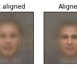
One important thing I found that helped is to align the images so the facial features overlap.
It helps the nets learn the variance in faces better, rather than waste their “representation power” on the shift between faces.
The following is some code to align face images using the excellent Dlib (python bindings) http://dlib.net. First I’m just using a standard face detector, and then using the facial fatures extractor I’m using that information for a complete alignment of the face.
After the alignment – I’m just having fun with the aligned dataset
Tag: opencv
As part of the computer vision class I’m teaching at SBU I asked students to implement a segmentation method based on SLIC superpixels. Here is my boilerplate implementation.
This follows the work I’ve done a very long time ago (2010) on the same subject.
For graph-cut I’ve used PyMaxflow: https://github.com/pmneila/PyMaxflow, which is very easily installed by just pip install PyMaxflow
The method is simple:
- Calculate SLIC superpixels (the SKImage implementation)
- Use markings to determine the foreground and background color histograms (from the superpixels under the markings)
- Setup a graph with a straightforward energy model: Smoothness term = K-L-Div between superpix histogram and neighbor superpix histogram, and Match term = inf if marked as BG or FG, or K-L-Div between SuperPix histogram and FG and BG.
- To find neighbors I’ve used Delaunay tessellation (from scipy.spatial), for simplicity. But a full neighbor finding could be implemented by looking at all the neighbors on the superpix’s boundary.
- Color histograms are 2D over H-S (from the HSV)
import cv2 | |
import numpy as np | |
import matplotlib.pyplot as plt | |
from skimage.segmentation import slic | |
from skimage.segmentation import mark_boundaries | |
from skimage.data import astronaut | |
from skimage.util import img_as_float | |
import maxflow | |
from scipy.spatial import Delaunay | |
# Calculate the SLIC superpixels, their histograms and neighbors | |
def superpixels_histograms_neighbors(img): | |
# SLIC | |
segments = slic(img, n_segments=500, compactness=20) | |
segments_ids = np.unique(segments) | |
# centers | |
centers = np.array([np.mean(np.nonzero(segments==i),axis=1) for i in segments_ids]) | |
# H-S histograms for all superpixels | |
hsv = cv2.cvtColor(img.astype('float32'), cv2.COLOR_BGR2HSV) | |
bins = [20, 20] # H = S = 20 | |
ranges = [0, 360, 0, 1] # H: [0, 360], S: [0, 1] | |
colors_hists = np.float32([cv2.calcHist([hsv],[0, 1], np.uint8(segments==i), bins, ranges).flatten() for i in segments_ids]) | |
# neighbors via Delaunay tesselation | |
tri = Delaunay(centers) | |
return (centers,colors_hists,segments,tri.vertex_neighbor_vertices) | |
# Get superpixels IDs for FG and BG from marking | |
def find_superpixels_under_marking(marking, superpixels): | |
fg_segments = np.unique(superpixels[marking[:,:,0]!=255]) | |
bg_segments = np.unique(superpixels[marking[:,:,2]!=255]) | |
return (fg_segments, bg_segments) | |
# Sum up the histograms for a given selection of superpixel IDs, normalize | |
def cumulative_histogram_for_superpixels(ids, histograms): | |
h = np.sum(histograms[ids],axis=0) | |
return h / h.sum() | |
# Get a bool mask of the pixels for a given selection of superpixel IDs | |
def pixels_for_segment_selection(superpixels_labels, selection): | |
pixels_mask = np.where(np.isin(superpixels_labels, selection), True, False) | |
return pixels_mask | |
# Get a normalized version of the given histograms (divide by sum) | |
def normalize_histograms(histograms): | |
return np.float32([h / h.sum() for h in histograms]) | |
# Perform graph cut using superpixels histograms | |
def do_graph_cut(fgbg_hists, fgbg_superpixels, norm_hists, neighbors): | |
num_nodes = norm_hists.shape[0] | |
# Create a graph of N nodes, and estimate of 5 edges per node | |
g = maxflow.Graph[float](num_nodes, num_nodes * 5) | |
# Add N nodes | |
nodes = g.add_nodes(num_nodes) | |
hist_comp_alg = cv2.HISTCMP_KL_DIV | |
# Smoothness term: cost between neighbors | |
indptr,indices = neighbors | |
for i in range(len(indptr)-1): | |
N = indices[indptr[i]:indptr[i+1]] # list of neighbor superpixels | |
hi = norm_hists[i] # histogram for center | |
for n in N: | |
if (n < 0) or (n > num_nodes): | |
continue | |
# Create two edges (forwards and backwards) with capacities based on | |
# histogram matching | |
hn = norm_hists[n] # histogram for neighbor | |
g.add_edge(nodes[i], nodes[n], 20-cv2.compareHist(hi, hn, hist_comp_alg), | |
20-cv2.compareHist(hn, hi, hist_comp_alg)) | |
# Match term: cost to FG/BG | |
for i,h in enumerate(norm_hists): | |
if i in fgbg_superpixels[0]: | |
g.add_tedge(nodes[i], 0, 1000) # FG - set high cost to BG | |
elif i in fgbg_superpixels[1]: | |
g.add_tedge(nodes[i], 1000, 0) # BG - set high cost to FG | |
else: | |
g.add_tedge(nodes[i], cv2.compareHist(fgbg_hists[0], h, hist_comp_alg), | |
cv2.compareHist(fgbg_hists[1], h, hist_comp_alg)) | |
g.maxflow() | |
return g.get_grid_segments(nodes) | |
if __name__ == '__main__': | |
img = img_as_float(astronaut()[::2, ::2]) | |
img_marking = cv2.imread("astronaut_marking.png") | |
centers, colors_hists, segments, neighbors = superpixels_histograms_neighbors(img) | |
fg_segments, bg_segments = find_superpixels_under_marking(img_marking, segments) | |
# get cumulative BG/FG histograms, before normalization | |
fg_cumulative_hist = cumulative_histogram_for_superpixels(fg_segments, colors_hists) | |
bg_cumulative_hist = cumulative_histogram_for_superpixels(bg_segments, colors_hists) | |
norm_hists = normalize_histograms(colors_hists) | |
graph_cut = do_graph_cut((fg_cumulative_hist, bg_cumulative_hist), | |
(fg_segments, bg_segments), | |
norm_hists, | |
neighbors) | |
plt.subplot(1,2,2), plt.xticks([]), plt.yticks([]) | |
plt.title('segmentation') | |
segmask = pixels_for_segment_selection(segments, np.nonzero(graph_cut)) | |
cv2.imwrite("output_segmentation.png", np.uint8(segmask * 255)) | |
plt.imshow(segmask) | |
plt.subplot(1,2,1), plt.xticks([]), plt.yticks([]) | |
img = mark_boundaries(img, segments) | |
img[img_marking[:,:,0]!=255] = (1,0,0) | |
img[img_marking[:,:,2]!=255] = (0,0,1) | |
plt.imshow(img) | |
plt.title("SLIC + markings") | |
plt.savefig("segmentation.png",bbox_inches='tight',dpi=96) |
Result
A small example on how to do Laplacian pyramid blending with an arbitrary mask.
Enjoy
Roy
# adapted from http://docs.opencv.org/3.0-beta/doc/py_tutorials/py_imgproc/py_pyramids/py_pyramids.html | |
import cv2 | |
import numpy as np | |
def Laplacian_Pyramid_Blending_with_mask(A, B, m, num_levels = 6): | |
# assume mask is float32 [0,1] | |
# generate Gaussian pyramid for A,B and mask | |
GA = A.copy() | |
GB = B.copy() | |
GM = m.copy() | |
gpA = [GA] | |
gpB = [GB] | |
gpM = [GM] | |
for i in xrange(num_levels): | |
GA = cv2.pyrDown(GA) | |
GB = cv2.pyrDown(GB) | |
GM = cv2.pyrDown(GM) | |
gpA.append(np.float32(GA)) | |
gpB.append(np.float32(GB)) | |
gpM.append(np.float32(GM)) | |
# generate Laplacian Pyramids for A,B and masks | |
lpA = [gpA[num_levels-1]] # the bottom of the Lap-pyr holds the last (smallest) Gauss level | |
lpB = [gpB[num_levels-1]] | |
gpMr = [gpM[num_levels-1]] | |
for i in xrange(num_levels-1,0,-1): | |
# Laplacian: subtarct upscaled version of lower level from current level | |
# to get the high frequencies | |
LA = np.subtract(gpA[i-1], cv2.pyrUp(gpA[i])) | |
LB = np.subtract(gpB[i-1], cv2.pyrUp(gpB[i])) | |
lpA.append(LA) | |
lpB.append(LB) | |
gpMr.append(gpM[i-1]) # also reverse the masks | |
# Now blend images according to mask in each level | |
LS = [] | |
for la,lb,gm in zip(lpA,lpB,gpMr): | |
ls = la * gm + lb * (1.0 - gm) | |
LS.append(ls) | |
# now reconstruct | |
ls_ = LS[0] | |
for i in xrange(1,num_levels): | |
ls_ = cv2.pyrUp(ls_) | |
ls_ = cv2.add(ls_, LS[i]) | |
return ls_ | |
if __name__ == '__main__': | |
A = cv2.imread("input1.png",0) | |
B = cv2.imread("input2.png",0) | |
m = np.zeros_like(A, dtype='float32') | |
m[:,A.shape[1]/2:] = 1 # make the mask half-and-half | |
lpb = Laplacian_Pyramid_Blending_with_mask(A, B, m, 5) | |
cv2.imwrite("lpb.png",lpb) |
Hello again!
After a long hiatus I’m back with an update. Recently I’ve been upgrading the Structure-from-Motion Toy Library (https://github.com/royshil/SfM-Toy-Library/) to OpenCV 3.x from OpenCV 2.4.x.
Using Poppler, of course!
Poppler is a very useful tool for handling PDF, so I’ve discovered lately. Having tried both muPDF and ImageMagick’s Magick++ and failed, Poppler stepped up to the challenge and paid off.
So here’s a small example of how work the API (with OpenCV, naturally):
1 2 3 4 5 6 7 8 9 10 11 12 13 14 15 16 17 18 19 20 21 22 23 24 25 26 27 28 29 30 31 32 33 34 | #include <iostream> #include <fstream> #include <sstream> #include <opencv2/opencv.hpp> #include <poppler-document.h> #include <poppler-page.h> #include <poppler-page-renderer.h> #include <poppler-image.h> using namespace cv; using namespace std; using namespace poppler; Mat readPDFtoCV( const string& filename, int DPI) { document* mypdf = document::load_from_file(filename); if (mypdf == NULL) { cerr << "couldn't read pdf\n" ; return Mat(); } cout << "pdf has " << mypdf->pages() << " pages\n" ; page* mypage = mypdf->create_page(0); page_renderer renderer; renderer.set_render_hint(page_renderer::text_antialiasing); image myimage = renderer.render_page(mypage,DPI,DPI); cout << "created image of " << myimage.width() << "x" << myimage.height() << "\n" ; Mat cvimg; if (myimage.format() == image::format_rgb24) { Mat(myimage.height(),myimage.width(),CV_8UC3,myimage.data()).copyTo(cvimg); } else if (myimage.format() == image::format_argb32) { Mat(myimage.height(),myimage.width(),CV_8UC4,myimage.data()).copyTo(cvimg); } else { cerr << "PDF format no good\n" ; return Mat(); } return cvimg; } |
All you have to do is give it the DPI (say you want to render in 100 DPI) and a filename.
Keep in mind it only renders the first page, but getting the other pages is just as easy.
That’s it, enjoy!
Roy.
Years ago I wanted to implement PTAM. I was young and naïve
Well I got a few moments to spare on a recent sleepless night, and I set out to implement the basic bootstrapping step of initializing a map with a planar object – no known markers needed, and then tracking it for augmented reality purposes.
So lately I’m into Optical Music Recognition (OMR), and a central part of that is doing staff line removal. That is when you get rid of the staff lines that obscure the musical symbols to make recognition much easier. There are a lot of ways to do it, but I’m going to share with you how I did it (fairly easily) with Hidden Markov Models (HMMs), which will also teach us a good lesson on this wonderfully useful approach.
OMR has been around for ages, and if you’re interested in learning about it [Fornes 2014] and [Rebelo 2012] are good summary articles.
The matter of Staff Line Removal has occupied dozens of researchers for as long as OMR exists; [Dalitz 2008] give a good overview. Basically the goal is to remove the staff lines that obscure the musical symbols, so they would be easier to recognize.
But, the staff lines are connected to the symbols, so simply removing them will cut up the symbols and make them hardly recognizable.
So let’s see how we could do this with HMMs.
I came across an extremely simple color balancing algorithm here. And I thought I’ll quickly transcode it to OpenCV.
Here’s the gist:
I wish to report of a number of tweaks and additions to the hand silhouette tracker I posted a while back. First is the ability for it to “snap” to the object using a simple Active Snake method, another is a more advanced resampling technique (the older tracker always resampled after every frame), and of a number of optimizations to increase the speed (tracker now runs at real-time on a single core).